Predict Taxi Fare with a BigQuery ML Forecasting Model — Google Cloud Platform GCP 實際操作實習手冊

Open BigQuery Console

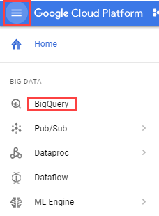
In the Google Cloud Console, select Navigation menu > BigQuery:

The Welcome to BigQuery in the Cloud Console message box opens. This message box provides a link to the quickstart guide and the release notes.

Click Done.

The BigQuery console opens.

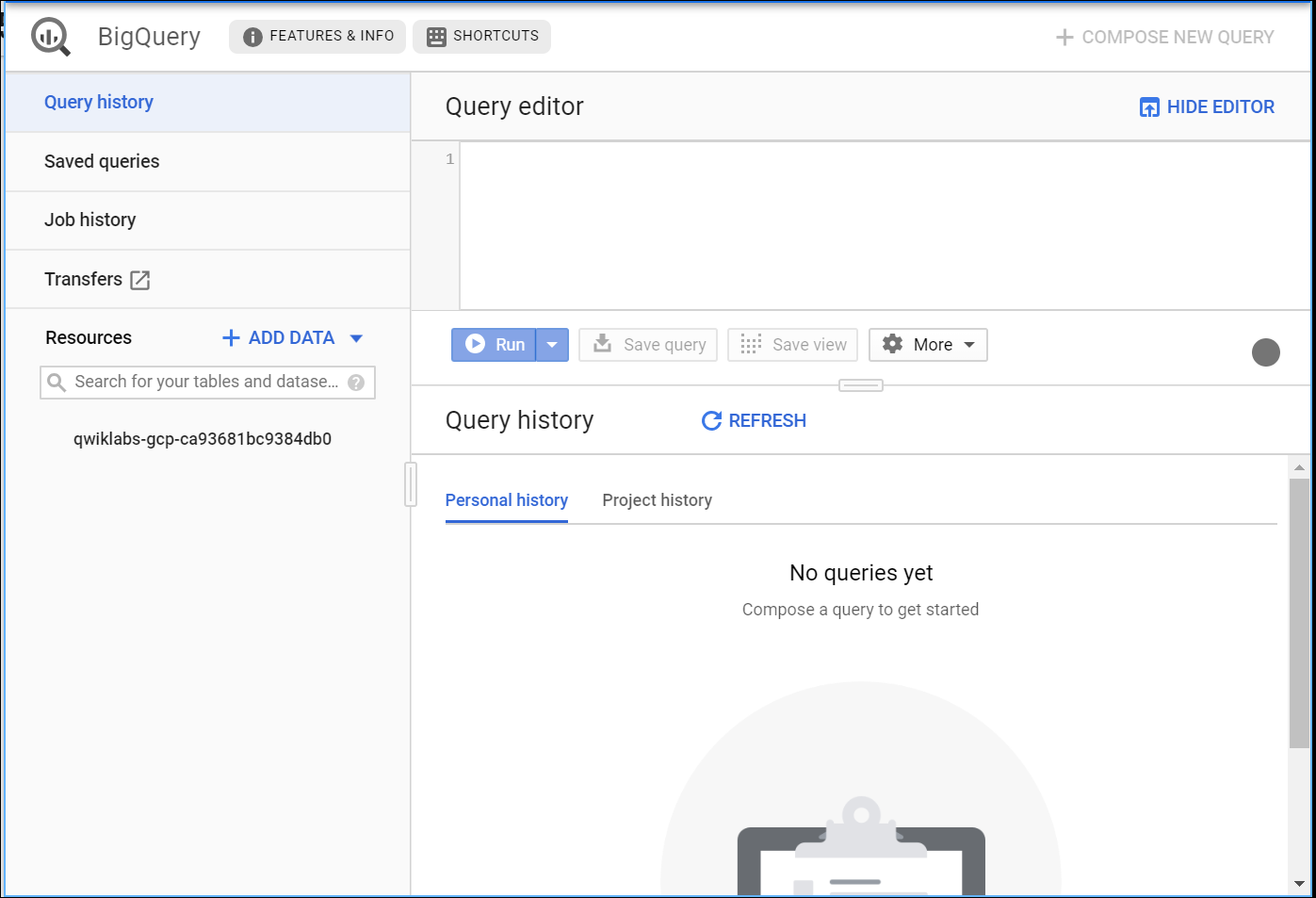
Explore NYC taxi cab data

Question: How many trips did Yellow taxis take each month in 2015?

Copy and paste the following SQL code into the Query Editor:

#standardSQL
SELECT
  TIMESTAMP_TRUNC(pickup_datetime,
    MONTH) month,
  COUNT(*) trips
FROM
  `bigquery-public-data.new_york.tlc_yellow_trips_2015`
GROUP BY
  1
ORDER BY
  1

Then click Run.

You should receive the following result:

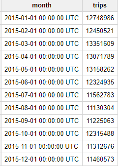
As we see, every month in 2015 had over 10 million NYC taxi trips—no small amount!

Replace the previous query with the following and then click Run:

#standardSQL
SELECT
  EXTRACT(HOUR
  FROM
    pickup_datetime) hour,
  ROUND(AVG(trip_distance / TIMESTAMP_DIFF(dropoff_datetime,
        pickup_datetime,
        SECOND))*3600, 1) speed
FROM
  `bigquery-public-data.new_york.tlc_yellow_trips_2015`
WHERE
  trip_distance > 0
  AND fare_amount/trip_distance BETWEEN 2
  AND 10
  AND dropoff_datetime > pickup_datetime
GROUP BY
  1
ORDER BY
  1

You should receive the following result:

During the day, the average speed is around 11-12 MPH; but at 5:00 AM the average speed almost doubles to 21 MPH. Intuitively this makes sense since there is likely less traffic on the road at 5:00 AM.

Identify an objective

You will now create a machine learning model in BigQuery to predict the price of a cab ride in New York City given the historical dataset of trips and trip data. Predicting the fare before the ride could be very useful for trip planning for both the rider and the taxi agency.

Select features and create your training dataset

The New York City Yellow Cab dataset is a public dataset provided by the city and has been loaded into BigQuery for your exploration. Browse the complete list of fields here and then preview the dataset to find useful features that will help a machine learning model understand the relationship between data about historical cab rides and the price of the fare.

Your team decides to test whether these below fields are good inputs to your fare forecasting model:

• Tolls Amount
• Fare Amount
• Hour of Day
• Pick up address
• Drop off address
• Number of passengers

Replace the query with the following:

#standardSQL
WITH params AS (
    SELECT
    1 AS TRAIN,
    2 AS EVAL
    ),

  daynames AS
    (SELECT ['Sun', 'Mon', 'Tues', 'Wed', 'Thurs', 'Fri', 'Sat'] AS daysofweek),

  taxitrips AS (
  SELECT
    (tolls_amount + fare_amount) AS total_fare,
    daysofweek[ORDINAL(EXTRACT(DAYOFWEEK FROM pickup_datetime))] AS dayofweek,
    EXTRACT(HOUR FROM pickup_datetime) AS hourofday,
    pickup_longitude AS pickuplon,
    pickup_latitude AS pickuplat,
    dropoff_longitude AS dropofflon,
    dropoff_latitude AS dropofflat,
    passenger_count AS passengers
  FROM
    `nyc-tlc.yellow.trips`, daynames, params
  WHERE
    trip_distance > 0 AND fare_amount > 0
    AND MOD(ABS(FARM_FINGERPRINT(CAST(pickup_datetime AS STRING))),1000) = params.TRAIN
  )

  SELECT *
  FROM taxitrips

Note a few things about the query:

1. The main part of the query is at the bottom (SELECT * from taxitrips).
2. taxitrips does the bulk of the extraction for the NYC dataset, with the SELECTcontaining your training features and label.
3. The WHERE removes data that you don't want to train on.
4. The WHERE also includes a sampling clause to pick up only 1/1000th of the data.
5. Define a variable called TRAIN so that you can quickly build an independent EVALset.

Now that you have a better understanding of this query's purpose, click Run.

You should receive a similar result:

What is the label (correct answer)?

total_fare is the label (what you will be predicting). You created this field out of tolls_amount and fare_amount, so you could ignore customer tips as part of the model as they are discretionary.

Create a BigQuery dataset to store models

In this section, you will create a new BigQuery dataset which will store your ML models.

1. In the left-hand Resources panel, select your Qwiklabs GCP Project ID.
2. Then on the right-hand side of the page, click CREATE DATASET.
3. In the Create Dataset dialog, enter in the following:

• For Dataset ID, type taxi.
• Leave the other values at their defaults.

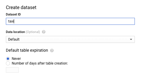
4. Then click Create dataset.

Select a BQML model type and specify options

Now that you have your initial features selected, you are now ready to create your first ML model in BigQuery.

There are several model types to choose from:

Model	Model Type	Label Data type	Example
Forecasting	linear_reg	Numeric value (typically an integer or floating point)	Forecast sales figures for next year given historical sales data.
Binary Classification	logistic_reg	0 or 1 for binary classification	Classify an email as spam or not spam given the context.
Multiclass Classification	logistic_reg	These models can be used to predict multiple possible values such as whether an input is "low-value", "medium-value", or "high-value". Labels can have up to 50 unique values.	Classify an email as spam, normal priority, or high importance.

Note: There are many additional model types used in Machine Learning (like Neural Networks and decision trees) and available using libraries like TensorFlow. At this time, BQML supports the three listed above. Follow the BQML roadmap for more information.

Enter the following query to create a model and specify model options, replacing -- paste the previous training dataset query here with the training dataset query you created earlier (omitting the #standardSQL line):

#standardSQL
CREATE or REPLACE MODEL taxi.taxifare_model
OPTIONS
  (model_type='linear_reg', labels=['total_fare']) AS
-- paste the previous training dataset query here

It will look something like this:

#standardSQL
CREATE or REPLACE MODEL taxi.taxifare_model
OPTIONS
  (model_type='linear_reg', labels=['total_fare']) AS

WITH params AS (
    SELECT
    1 AS TRAIN,
    2 AS EVAL
    ),

  daynames AS
    (SELECT ['Sun', 'Mon', 'Tues', 'Wed', 'Thurs', 'Fri', 'Sat'] AS daysofweek),

  taxitrips AS (
  SELECT
    (tolls_amount + fare_amount) AS total_fare,
    daysofweek[ORDINAL(EXTRACT(DAYOFWEEK FROM pickup_datetime))] AS dayofweek,
    EXTRACT(HOUR FROM pickup_datetime) AS hourofday,
    pickup_longitude AS pickuplon,
    pickup_latitude AS pickuplat,
    dropoff_longitude AS dropofflon,
    dropoff_latitude AS dropofflat,
    passenger_count AS passengers
  FROM
    `nyc-tlc.yellow.trips`, daynames, params
  WHERE
    trip_distance > 0 AND fare_amount > 0
    AND MOD(ABS(FARM_FINGERPRINT(CAST(pickup_datetime AS STRING))),1000) = params.TRAIN
  )

  SELECT *
  FROM taxitrips

Next, click Run to train your model.

Wait for the model to train (5 - 10 minutes).

After your model is trained, you will see the message "This was a CREATE operation. Results will not be shown" which indicates that your model has been successfully trained.

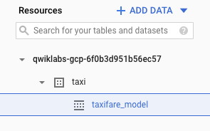
Look inside your taxi dataset and confirm taxifare_model now appears:

Next, you will evaluate the performance of the model against new unseen evaluation data.

Evaluate classification model performance

Select your performance criteria

For linear regression models you want to use a loss metric like Root Mean Square Error (RMSE). You want to keep training and improving the model until it has the lowest RMSE.

In BQML, mean_squared_error is a queryable field when evaluating your trained ML model. Add a SQRT() to get RMSE.

Now that training is complete, you can evaluate how well the model performs with this query using ML.EVALUATE. Copy and paste the following into the query editor and click Run:

#standardSQL
SELECT
  SQRT(mean_squared_error) AS rmse
FROM
  ML.EVALUATE(MODEL taxi.taxifare_model,
  (

  WITH params AS (
    SELECT
    1 AS TRAIN,
    2 AS EVAL
    ),

  daynames AS
    (SELECT ['Sun', 'Mon', 'Tues', 'Wed', 'Thurs', 'Fri', 'Sat'] AS daysofweek),

  taxitrips AS (
  SELECT
    (tolls_amount + fare_amount) AS total_fare,
    daysofweek[ORDINAL(EXTRACT(DAYOFWEEK FROM pickup_datetime))] AS dayofweek,
    EXTRACT(HOUR FROM pickup_datetime) AS hourofday,
    pickup_longitude AS pickuplon,
    pickup_latitude AS pickuplat,
    dropoff_longitude AS dropofflon,
    dropoff_latitude AS dropofflat,
    passenger_count AS passengers
  FROM
    `nyc-tlc.yellow.trips`, daynames, params
  WHERE
    trip_distance > 0 AND fare_amount > 0
    AND MOD(ABS(FARM_FINGERPRINT(CAST(pickup_datetime AS STRING))),1000) = params.EVAL
  )

  SELECT *
  FROM taxitrips

  ))

You are now evaluating the model against a different set of taxi cab trips with your params.EVAL filter.

After the model runs, review your model results (your model RMSE value will vary slightly).

Row	rmse
1	9.477056435999074

After evaluating your model you get a RMSE of $9.47. Knowing whether or not this loss metric is acceptable to productionalize your model is entirely dependent on your benchmark criteria, which is set before model training begins. Benchmarking is establishing a minimum level of model performance and accuracy that is acceptable.

Test Completed Task

Click Check my progress to verify your performed task. If you have completed the task successfully, you will be granted with an assessment score.

Evaluate the classification model performance

Predict taxi fare amount

Next you will write a query to use your new model to make predictions. Copy and paste the following into the Query editor and click Run:

#standardSQL
SELECT
*
FROM
  ml.PREDICT(MODEL `taxi.taxifare_model`,
   (

 WITH params AS (
    SELECT
    1 AS TRAIN,
    2 AS EVAL
    ),

  daynames AS
    (SELECT ['Sun', 'Mon', 'Tues', 'Wed', 'Thurs', 'Fri', 'Sat'] AS daysofweek),

  taxitrips AS (
  SELECT
    (tolls_amount + fare_amount) AS total_fare,
    daysofweek[ORDINAL(EXTRACT(DAYOFWEEK FROM pickup_datetime))] AS dayofweek,
    EXTRACT(HOUR FROM pickup_datetime) AS hourofday,
    pickup_longitude AS pickuplon,
    pickup_latitude AS pickuplat,
    dropoff_longitude AS dropofflon,
    dropoff_latitude AS dropofflat,
    passenger_count AS passengers
  FROM
    `nyc-tlc.yellow.trips`, daynames, params
  WHERE
    trip_distance > 0 AND fare_amount > 0
    AND MOD(ABS(FARM_FINGERPRINT(CAST(pickup_datetime AS STRING))),1000) = params.EVAL
  )

  SELECT *
  FROM taxitrips

));

Now you will see the model's predictions for taxi fares alongside the actual fares and other features for those rides. Your results should look similar to those below:

Improving the model with Feature Engineering

Building Machine Learning models is an iterative process. Once we have evaluated the performance of our initial model, we often go back and prune our features and rows to see if we can get an even better model.

Filtering the training dataset

Let's view the common statistics for taxi cab fares. Copy and paste the following into the Query editor and click Run:

SELECT
  COUNT(fare_amount) AS num_fares,
  MIN(fare_amount) AS low_fare,
  MAX(fare_amount) AS high_fare,
  AVG(fare_amount) AS avg_fare,
  STDDEV(fare_amount) AS stddev
FROM
`nyc-tlc.yellow.trips`
# 1,108,779,463 fares

You should receive a similar output:

As you can see, there are some strange outliers in our dataset (negative fares or fares over $50,000). Let's apply some of our subject matter expertise to help the model avoid learning on strange outliers.

Let's limit the data to only fares between $6 and $200. Copy and paste the following into the Query editor and click Run:

SELECT
  COUNT(fare_amount) AS num_fares,
  MIN(fare_amount) AS low_fare,
  MAX(fare_amount) AS high_fare,
  AVG(fare_amount) AS avg_fare,
  STDDEV(fare_amount) AS stddev
FROM
`nyc-tlc.yellow.trips`
WHERE trip_distance > 0 AND fare_amount BETWEEN 6 and 200
# 843,834,902 fares

You should receive a similar output:

That's a little bit better. While you're at, let's limit the distance traveled so you're really focusing on New York City.

Copy and paste the following into the Query editor and click Run:

SELECT
  COUNT(fare_amount) AS num_fares,
  MIN(fare_amount) AS low_fare,
  MAX(fare_amount) AS high_fare,
  AVG(fare_amount) AS avg_fare,
  STDDEV(fare_amount) AS stddev
FROM
`nyc-tlc.yellow.trips`
WHERE trip_distance > 0 AND fare_amount BETWEEN 6 and 200
    AND pickup_longitude > -75 #limiting of the distance the taxis travel out
    AND pickup_longitude < -73
    AND dropoff_longitude > -75
    AND dropoff_longitude < -73
    AND pickup_latitude > 40
    AND pickup_latitude < 42
    AND dropoff_latitude > 40
    AND dropoff_latitude < 42
    # 827,365,869 fares

You should receive a similar output:

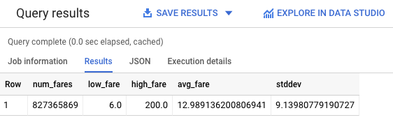
You still have a large training dataset of over 800 million rides for our new model to learn from. Let's re-train the model with these new constraints and see how well it performs.

Retraining the model

Let's call our new model taxi.taxifare_model_2 and retrain our linear regression model to predict total fare. You'll note that you've also added a few calculated features for the Euclidean distance (straight line) between the pick up and drop off.

Copy and paste the following into the Query editor and click Run:

CREATE OR REPLACE MODEL taxi.taxifare_model_2
OPTIONS
  (model_type='linear_reg', labels=['total_fare']) AS


WITH params AS (
    SELECT
    1 AS TRAIN,
    2 AS EVAL
    ),

  daynames AS
    (SELECT ['Sun', 'Mon', 'Tues', 'Wed', 'Thurs', 'Fri', 'Sat'] AS daysofweek),

  taxitrips AS (
  SELECT
    (tolls_amount + fare_amount) AS total_fare,
    daysofweek[ORDINAL(EXTRACT(DAYOFWEEK FROM pickup_datetime))] AS dayofweek,
    EXTRACT(HOUR FROM pickup_datetime) AS hourofday,
    SQRT(POW((pickup_longitude - dropoff_longitude),2) + POW(( pickup_latitude - dropoff_latitude), 2)) as dist, #Euclidean distance between pickup and drop off
    SQRT(POW((pickup_longitude - dropoff_longitude),2)) as longitude, #Euclidean distance between pickup and drop off in longitude
    SQRT(POW((pickup_latitude - dropoff_latitude), 2)) as latitude, #Euclidean distance between pickup and drop off in latitude
    passenger_count AS passengers
  FROM
    `nyc-tlc.yellow.trips`, daynames, params
WHERE trip_distance > 0 AND fare_amount BETWEEN 6 and 200
    AND pickup_longitude > -75 #limiting of the distance the taxis travel out
    AND pickup_longitude < -73
    AND dropoff_longitude > -75
    AND dropoff_longitude < -73
    AND pickup_latitude > 40
    AND pickup_latitude < 42
    AND dropoff_latitude > 40
    AND dropoff_latitude < 42
    AND MOD(ABS(FARM_FINGERPRINT(CAST(pickup_datetime AS STRING))),1000) = params.TRAIN
  )

  SELECT *
  FROM taxitrips

It may take a couple minutes to retrain the model. You can move onto the next step when you receive the following message in the Console:

Evaluate the new model

Now that our linear regression model has been optimized, let's evaluate the dataset with it and see how it performs. Copy and paste the following into the Query editor and click Run:

SELECT
  SQRT(mean_squared_error) AS rmse
FROM
  ML.EVALUATE(MODEL taxi.taxifare_model_2,
  (

  WITH params AS (
    SELECT
    1 AS TRAIN,
    2 AS EVAL
    ),

  daynames AS
    (SELECT ['Sun', 'Mon', 'Tues', 'Wed', 'Thurs', 'Fri', 'Sat'] AS daysofweek),

  taxitrips AS (
  SELECT
    (tolls_amount + fare_amount) AS total_fare,
    daysofweek[ORDINAL(EXTRACT(DAYOFWEEK FROM pickup_datetime))] AS dayofweek,
    EXTRACT(HOUR FROM pickup_datetime) AS hourofday,
    SQRT(POW((pickup_longitude - dropoff_longitude),2) + POW(( pickup_latitude - dropoff_latitude), 2)) as dist, #Euclidean distance between pickup and drop off
    SQRT(POW((pickup_longitude - dropoff_longitude),2)) as longitude, #Euclidean distance between pickup and drop off in longitude
    SQRT(POW((pickup_latitude - dropoff_latitude), 2)) as latitude, #Euclidean distance between pickup and drop off in latitude
    passenger_count AS passengers
  FROM
    `nyc-tlc.yellow.trips`, daynames, params
WHERE trip_distance > 0 AND fare_amount BETWEEN 6 and 200
    AND pickup_longitude > -75 #limiting of the distance the taxis travel out
    AND pickup_longitude < -73
    AND dropoff_longitude > -75
    AND dropoff_longitude < -73
    AND pickup_latitude > 40
    AND pickup_latitude < 42
    AND dropoff_latitude > 40
    AND dropoff_latitude < 42
    AND MOD(ABS(FARM_FINGERPRINT(CAST(pickup_datetime AS STRING))),1000) = params.EVAL
  )

  SELECT *
  FROM taxitrips

  ))

You should receive a similar output:

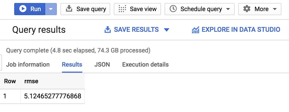
As you see, you've now gotten the RMSE down to: +-$5.12 which is significantly better than +-$9.47 for your first model.

Since RSME defines the standard deviation of prediction errors, we see that the retrained linear regression made our model a lot more accurate.

Other datasets to explore

You can use this below link to bring in the bigquery-public-dataproject if you want to explore modeling on other datasets like forecasting fares for Chicago taxi trips:

https://bigquery.cloud.google.com/table/bigquery-public-data::chicago_taxi_trips.taxi_trips